Embedded IA for IoT
Descriptive Part
The goal of this course was to gain solid foundations in machine learning and IA in general. The objectives included:
- understanding of the characteristics of supervised and unsupervised learning problems, as well as the basic methods and algorithms used to address them.
- AI at the edge and the optimization techniques required to embed AI algorithms effectively.
- Use Python libraries to solve real-world problems (with IoT data).
Technical Part
Introduction
Machine learning is a subset of the vast and electric world of Artificial Intelligence. It focuses on the development of algorithms that can learn from and make predictions on data.
Machine Learning for IoT focuses on creating models that can operate efficiently on devices with limited resources, such as microcontrollers, to process and analyze data locally (on the edge).
Artificial Intelligence > Machine Learning > Deep Learning
Resource Constraints in Edge AI
- Very low processing power and memory.
- Use of Digital Signal Processors (DSP) or Neural Processing Units (NPU) to optimize performance and efficiency.
- Limited energy availability, necessitating energy-efficient algorithms and hardware.
- Real-time processing requirements, demanding low-latency solutions.
Machine Learning for the Innovative Project
To add a bit of context on the matter, our interdisciplinary project aim to detect water leaks using a distributed network of sensors (WSN), each equipped with an ESP32 and a LoRa module for communication. These sensors transmit a payload consisting of metrics (frequency and harmonic data, timestamps, etc…) and edge computing analysis preliminary results (output of small machine learning models). Our LoRa module (SX1278) operate on frequencies ranging from 410MHz to 525MHz and is designed for low power consumption and limited bandwidth. Without any security features each sensor node is vulerable to every attack imaginable (replay attacks, data tempering, eavesdropping…). Consequently it is necessary for the project to implement a security solution that protects data integrity and confidentiality without introducing too much overhead.
Supervised Approach: Support Vector Machine
Link to the repository: GitHub Repository
Support Vector Machine Principle
Support Vector Machine or SVM is a supervised machine learning technique used to classify data by finding the best hyperplane that separates different categories (class). The main idea behind SVM is it aims to maximize the distance (margin) between the hyperplane and the nearest data points, helping ensure that the classification is robust because the data is well split. SVM works very well for linear problems but can also handle non-linear ones by using kernels, which are essentially mathematical functions that map data into a higher dimension where it becomes easier to separate.
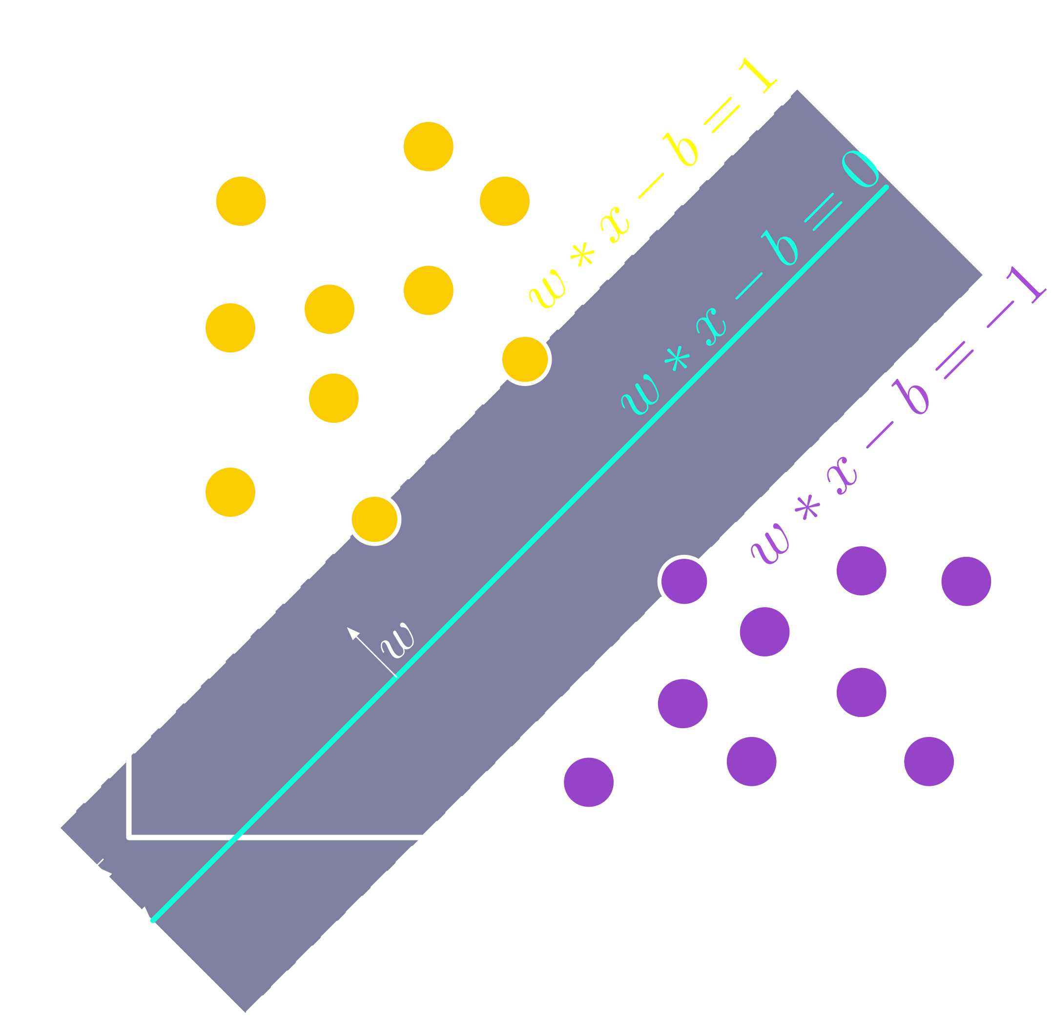 SVM Principle [source: Wikipedia]
In a nutshell, SVM tries to draw the most optimal line or surface that divides the data into categories while keeping the line as far away as possible from the closest point of each cluster of categories.
Mathematical Hints
Equation of the Hyperplane
In 2D, a line can be written as:
$$ y = wx + b $$
where $w$ is the slope, and $b$ is the y-intercept. This principle generalizes to a hyperplane in higher dimensions, but for obvious reasons, a line is simpler to visualize (one can only dream of visualizing a 42-dimension hyperplane). The goal of SVM is to find the best $w$ and $b$ that maximizes the separation margin.
Margin Maximization
The margin is the distance between the hyperplane and the closest points from each class (the support vectors). SVM maximizes this margin, which can be expressed as:
$$ \text{Margin} = \frac{2}{|w|} $$
where $|w|$ is the amplitude (length) of the vector $w$.
Constraint for Classification
SVM ensures that every data point is on the correct side of the margin. For a data point $x_i$ with a label $y_i \in {-1, 1}$, the constraint is:
$$ y_i \left( w \cdot x_i + b \right) \geq 1 $$
This means that points labeled $+1$ ($y_i = 1$) are on one side of the hyperplane, and points labeled $-1$ ($y_i = -1$) are on the other side.
Kernel when Things Go Non-linear
For non-linear problems, SVM applies a kernel function to transform the data into a higher-dimensional space where a hyperplane can separate them. For example, a simple kernel function might be:
$$ K(x_i, x_j) = \left( x_i \cdot x_j \right)^2 $$
Summary:
- The hyperplane is defined as $w \cdot x + b = 0$.
- All points satisfy the condition $y_i \left( w \cdot x_i + b \right) \geq 1$.
- The margin $\frac{2}{|w|}$ is maximized when training the model to obtain the best classification.
Implementation: Collect the Samples
In order to train the model, two distinct datasets were created: one representing leak acoustic signals and the other one without acoustic signals. Each dataset was composed of a 10-second spectrogram sample under the two scenarios. The data was collected using a serial connection to a WAL Node, and the raw FFT data was saved into CSV files.
Once the data was collected, it was displayed in a friendly spectrogram manner as follows to check for data integrity:
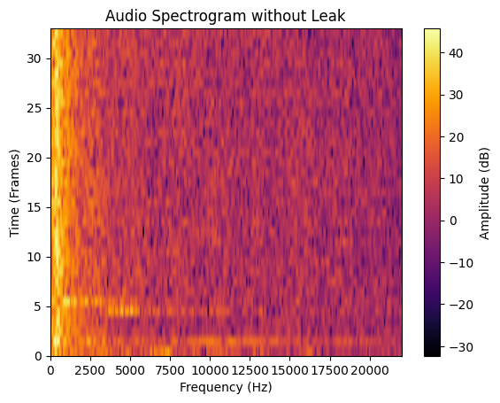 No Leak 10s Spectrogram Dataset
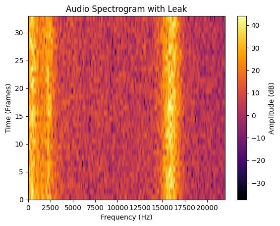 Leak 10s Spectrogram Dataset
Training the Model
A Support Vector Machine (SVM) was implemented to classify audio data into two categories: “Leak” and “No Leak”. After collecting the data, it was loaded, labeled, and combined for later processing.
The combined dataset was split into training and testing sets to evaluate the model’s performance. Features were standardized using a StandardScaler to ensure that all features contributed equally to the model. An SVM classifier with a linear kernel was trained on the training data.
After training, predictions were made on the test set, and the classifier’s performance was evaluated using the following classification report and confusion matrix:
| Class | Precision | Recall | F1-Score | Support |
|---|---|---|---|---|
| 0 | 1.00 | 1.00 | 1.00 | 7 |
| 1 | 1.00 | 1.00 | 1.00 | 7 |
| Accuracy | 1.00 | 14 | ||
| Macro Avg | 1.00 | 1.00 | 1.00 | 14 |
| Weighted Avg | 1.00 | 1.00 | 1.00 | 14 |
Classification Report
The classification report shows very good precision, recall, and F1-score for both classes, indicating that the model correctly identified all instances of “Leak” and “No Leak” in the test set. This demonstrates that the model is highly accurate and performs well on the dataset.
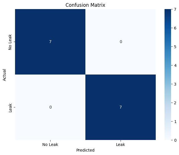 Confusion Matrix of the Trained SVM Model
Testing the Model
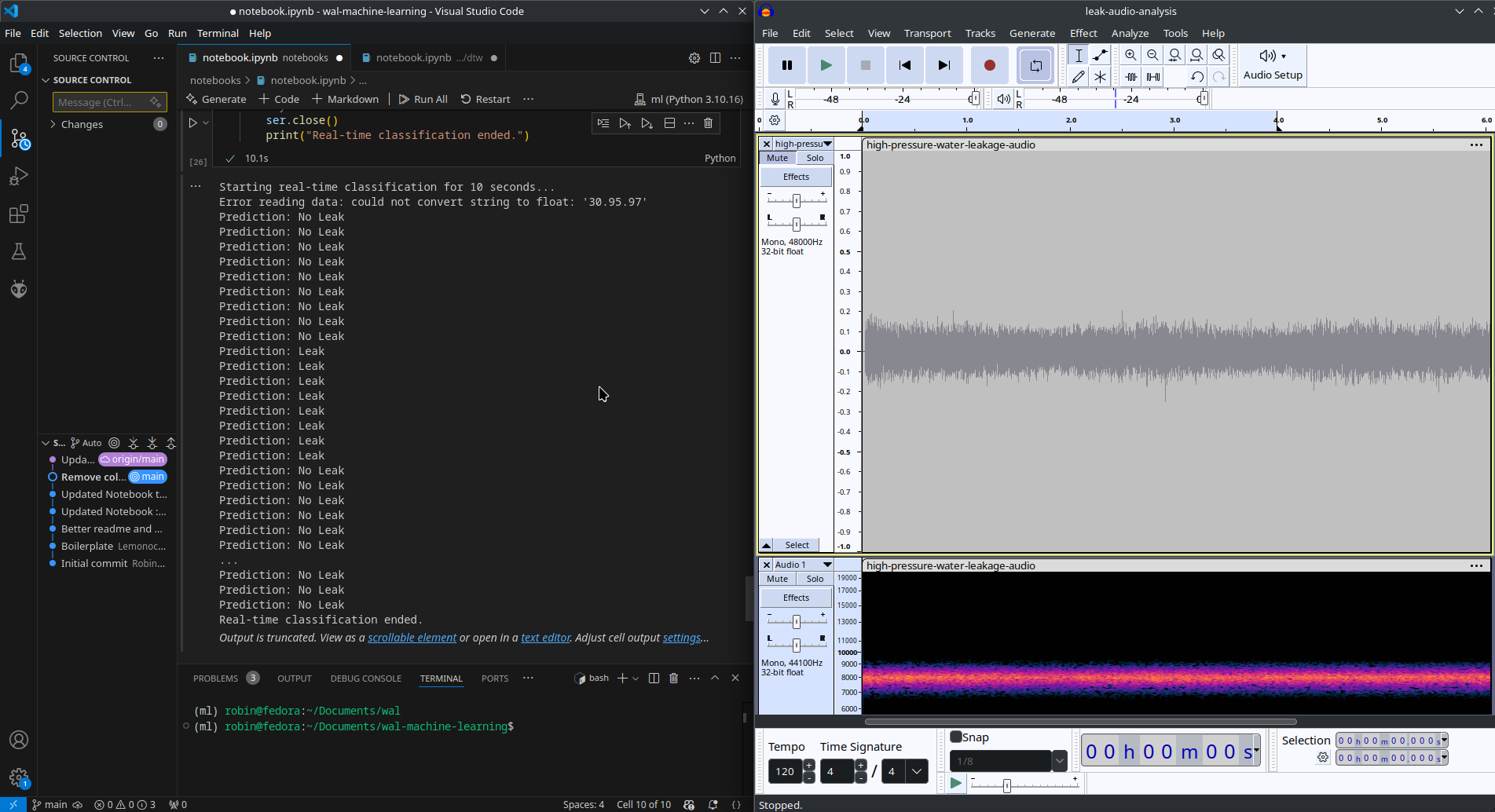 Left: Testing Script | Right: Audacity with Leak Audio
The model performs very well; it detects leaks even with very low amplitudes.
Analytical Part
This course was a very valuable and enjoyable experience. From the start the content was well-organized and made the complex topics easy to understand, I found the practical labs on Jupyter Notebooks very interesting, well-structured and this helkped me quickly learn new concepts. Learning how to optimize AI models to run on microcontrollers was particularly useful because we wanted to implement the same edge machine learning principles to our water leak detection inovative project. The only small regret is that we didn’t had the time to integrate and test the pruned/compressed model onto the development board during the labs. However, I plan to try it on my own as I have AI development board (Luckfox Pico Mini) from previous projects.
Overall, this course was very valuable. It gave me new skills, new interests, and the keys to apply machine learning techniques to personnal projects. I will keep learning and working on more projects in this field in the future.